

To provide a better understanding of the interpretation and limitations of space imagery, this appendix presents a brief survey of relevant principles of remote sensing and of those spaceborne sensors that provide images in this book (Table A-l). For a more in depth discussion of remote sensing, the reader is referred to Lillesand and Kieffer (1979), Lintz and Simonett (1976), Sabins (1978), Short (1982), Siegal and Gillespie (1980), and the second edition of the Manual of Remote Sensing (1983).
| Vehicle/Sensor | Spectral Bands (Ám) | Nominal Spatial Resolution (m) | Areal Coverage (km) | Frequency of Coverage | Data Center |
|---|---|---|---|---|---|
| Landsat 1, 2, 3, 4, 5/MSS | 0.5-0.6 0.6-0.7 0.7-0.8 0.8-1.1 | 79 | 34 000 km2 | Once every 18 days | EROS Data Center (EDC) |
| Landsat 3 RBV | 0.50-0.75 | 30 | 98 x 98 km | EDC | |
| Landsat 4, 5/TM | 0.45-0.52 0.52-0.60 0.63-0.69 0.76-0.90 1.55-1.75 2.08-2.30 10.40-12.55 | 30 | 185 x 185 km | 16 days | EDC |
| Heat Capacity Mapping Mission (HCMM) | 0.5-1.1 10.5-12.5 | 500 600 | 700-km Swath | 3 days | NASA/GSFC |
| Seasat SAR | 1.35 GHz (L-Band) | 25 | 100-km Swath | As scheduled | JPL/NOAA |
| STS (Shuttle) SIR-A | L-Band | 25-100 | 100-200-km Swath | As scheduled | JPL/NOAA |
| Tiros N/AVHRR | 4.5 Visible Bands, IR Thermal IR | 1100-4000 | Subcontinental | 12-24 hr | NOAA/NESS |
| Large-Format Camera | Panchromatic,
Stereo | 10 | Continental (480 x 180 km) | As scheduled | EDC/NSSDC |
REMOTE SENSING AND ELECTROMAGNETIC RADIATION
Remote sensing as a technology refers to the acquisition of data and derivative information about objects, classes, or materials located at some distance from the sensors by sampling radiation from selected regions (wavebands) of the electromagnetic (EM) spectrum. For sensors mounted on moving platforms (e.g., aircraft and satellites) operating in or above the Earth┤s atmosphere, the principal sensing regions are in the visible, reflected near-infrared, thermal infrared, and microwave/radar regions of the EM spectrum (Figure A-l). The particular wavelengths (or frequencies) detectable by visible/infrared sensors depend in large measure on the extent to which the waveband radiation is absorbed, scattered, or otherwise modified by the atmosphere ("windows of transparency" concept). The radiation measured from space platforms is usually secondary in that it is reflected or emitted energy generated from molecular interactions between incoming radiation (irradiance) and the Earth material being sensed. Common primary energy sources include the Sun or active radiation-generating devices such as radar; sensed thermal radiation from the Earth┤s surface results from both internal heat sources and the heating effect of solar radiation. Because most materials absorb radiation over the sensed parts of the EM spectrum, only fractions of the incoming radiation (typically, 1/20th (for water) to 4/5ths (sand) in the reflected region) are returned to the sensor.
| Figure A.1. The electromagnetic spectrum, atmospheric windows and spectral operating range of sensors; modified from R. Colwell (upper diagram) and from Remote Sensing of Environment. J. Lintz, Jr., and D.S. Simonett (Eds.), 1976, with permission of the publisher, Addison-Wesley, Reading, Massachusetts (lower diagram, E). |  |
|---|
The spectral character of the source radiation depends on how it is generated. A spectral distribution plot shows the variation with wavelength of irradiance levels, usually measured as intensity or power functions (illustrated for solar irradiance in Figure A-2). This distribution is initially modified as incoming radiation interacts with the atmosphere. It is then further changed through interaction with the surficial materials (to depths ranging from micrometers to a few meters, depending on wavelength), and the returned fraction is altered once more as it passes back through the atmosphere. Finally, the sensor itself modifies the returned radiation according to the response characteristics of the radiation-sensitive detectors. The end result is a spectral signature for each sampled section of the sensed surface, which is made by plotting the intensity or power variations of the final signal as a function of wavelength (Figure A-3). For the wavebands commonly used, the greatest modification is imparted by the interactions involving the ground materials, so that the signature is generally diagnostic of the particular substances or of objects composed of them. Targets of interest at the Earth┤s surface are usually an intimate mix of several materials (e.g., soil clays and rock particles, as well as water, air, and organic substances) or even several classes of materials such as soil plus trees plus grass plus manmade objects that are grouped together in an area of the ground. The size of the sampled area (target) is specified by the spatial resolution limit of the sensor (its instantaneous field of view as determined by the sensor┤s optics, electronics, etc.). On an image, this "area" is represented by the picture element (called a pixel); the pixel size for a Landsat Multispectral Scanner (MSS) scene is 79 m, and each full scene (for a band) is made up of 7.5 million pixels.
| Figure A.2. Solar irradiation curves, showing location of atmospheric absorption bands; from Handbook of Geophysics and Space Environments, S. Valley (Ed.),copyright® 1965 McGraw-Hill (published with permission of McGraw-Hill Brook Company). |  |
|---|
| Figure A.3. Reflectance spectra of Wyoming rock stratigraphic units. |  |
|---|
Spectral signatures obtained with a spectrometer, which uses a grating or prism to disperse a radiation continuum into discrete wavelengths, appear as continuous plots. More commonly, the detector/counter system operating in a moving sensor is capable of measuring only the radiation distributed over a finite wavelength interval or band. Band limits are determined by the transmission characteristics of a filter that passes only radiation of certain wavelengths. The detector integrates the distribution of spectroradiances into a single intensity/power value. If the radiation distribution is sampled at several intervals, the plots of these single values for their respective wavebands resemble a histogram (Figure A-4) that crudely approximates the spectrometer-produced signature. The more spectral bands sampled over a given spectral region, the closer the resultant signature will be to the characteristic signature of the object or material sensed.
REMOTE SENSING INSTRUMENTATION
The most common types of remote sensors are radiometers, multispectral scanners, spectrometers, and film cameras. The first two convert radiation (photons) emanating from each surface target into electrical signals whose magnitudes are proportional to the spectroradiances in the intervals (bands) sensed. The surface is usually sampled sequentially, as by a mirror scanning from side to side while the sensor moves forward on its platform. Each pixel contributes the collective radiation from the materials within it to the record as a single discrete quantity so that the converted signal is a measure of the combined ground target variation from one successive pixel area to the next. After being recorded, the signals can be played back into a device that generates a sweeping light beam whose intensity varies in proportion to the photon variations from pixel to pixel. The beam output is, in a sense, a series of light pulses, each equivalent to an average value for an individual ground target. Because the signal pulses were collected as an array of XY space in relation to their successively sensed target positions, the individual values can be displayed as a sequential series of points (pixels) of varying intensity. The image display may be on a television monitor, a film (pixels are represented by diffuse clusters of silver grains), or a sheet of paper on which pixel intensities are indicated by alphanumeric characters or by spots of variable densities or sizes (exemplified by a newspaper photograph). Any of these displays produces an image of the sensed scene comprising the variations in tonal densities of the different objects or classes within it in their correct relative positions. Normally, scanning spectrometers must dwell on a single target long enough for the full spectral interval to be traversed and hence cannot be operated from a moving platform unless the target is tracked (as was done by an astronaut on Skylab). This type of spectrometer presents the spectral signature as a continuous curve on a strip chart or plate. Fixed prism or grating spectrometers usually show discrete spectral wavelengths as a dispersed sequence of lines (images of a slit aperture). The Jet Propulsion Laboratory has developed an airborne imaging spectrometer that uses a slit to pass radiation from the ground onto a multilinear array charge-coupled detector (CCD) to sense successive areas along a moving track. The film camera differs from the sequential sensor types in that it allows the radiation from all surface targets sensed at the same instant to strike the film (recorder) simultaneously in their correct positions as determined by the optics of the system.
| Figure A.4. Relative densities of ground class MSS signatures of nine cover types in the Choptank River, Maryland, area. |  |
|---|
A set of multispectral images is produced by breaking the image-forming radiation into discrete spectral intervals through the use of waveband filters (or other light dispersion or selection devices). If a surface material has high reflectance or emittance in some given interval, it will be recorded as a light (bright) tone on a positive film-based image. Conversely, a dark tone represents a low reflectance or emittance. Because the same material normally has varying values of reflectance or emittance in different spectral regions, it will produce some characteristic gray level (on film) in the image for each particular waveband. Different materials give rise to different gray levels in any set of waveband images, thus creating the varying tonal patterns that spatially define classes, objects, or features. Multispectral images of the same scene are characterized by different tonal levels for the various classes from one band to the next.
REMOTE SENSING DATA DISPLAYS
Before Landsat and similar multispectral systems were developed, the principal remote sensing data displays were nearly always aerial photographs. Aerial cameras typically employ panchromatic films that use the visible region of the spectrum from about 0.40 to 0.70 micrometers (Ám). Use of a yellow haze (minus blue) filter, which prevents energy transmission below 0.51 Ám, narrows the actual waveband interval to 0.51 to 0.70 Ám in black and white aerial photography. Color aerial photographs are recorded on natural color or false-color infrared film. These operate on the color subtraction principle, in which the three color substrates or layers of a negative on development are yellow, magenta, and cyan, being sensitive to blue, green, and red light, respectively. However, when producing a "color composite" from individual waveband images, the color additive principle applies. Three such images are needed to make a multispectral color composite. Multiband photography utilizes several cameras, each consisting of a bore-sighted lens and a color filter that transmits a specific spectral interval or band through the optical train onto black and white film.
For each band, the film records the scene objects as various gray tones related to the visible colors (or other radiation) variably transmitted and absorbed by the particular filter. Suppose two objects, one red and the other green, are photographed by three bore-sighted cameras. Each cameraÁs lens would be focused on its own film, with one fronted by a blue filter, the second by a green filter, and the third by a red filter. When all three lens shutters are triggered together, light from the red object (mostly in the 0.6to 0.7-Ám interval) will only pass through the red filter (being absorbed to varying extents by the blue and green filters). In the red filter camera, the shape of the object is reproduced as a light-toned pattern set off against dark (equivalent to non-red) surroundings. For cameras that record this object through green and blue filters, the red light object is absorbed, reproducing its presence on film as a dark tone. The green object is likewise recorded as light-toned only on the green filter/film combination. Obviously, a blue object, if in the scene, would have appeared in light tones only on the blue filter/film product. Non-primary colors would likewise be rendered as various gray tones in the three images, at levels depending on their relative transmission through each filter (e.g., yellow light normally will be only partially absorbed by red and green filters).
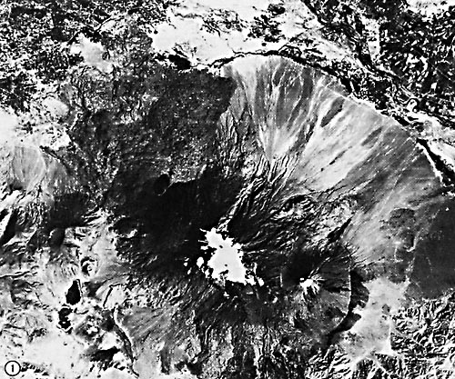
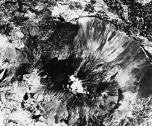
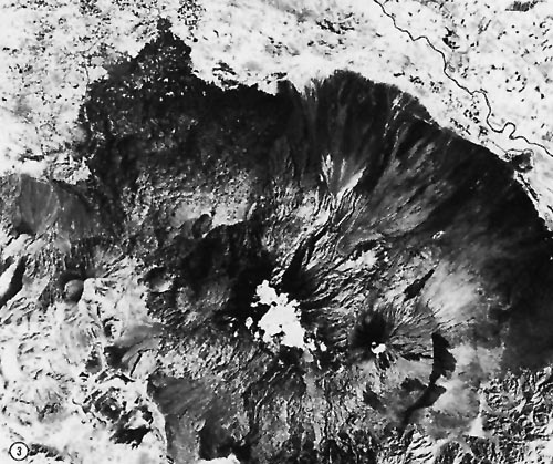
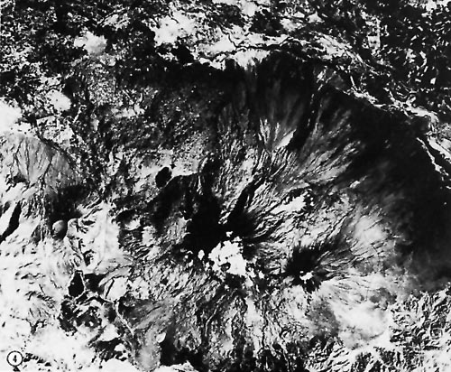
| Figure A.5. Computer-enhanced subscenes of the Thematic Mapper image of Mount Ararat in eastern Turkey (see Plate V-17) illustrating different bands and color-composite images: (1) Band 2; (2) Band 3; (3) Band 4; (4) Band 5; (5) Bands 2 (blue), 3 (green), and 4 (red); (6) Bands 1 (blue), 4 (green), and 5 (red). | |
|---|---|
 |  |
 |  |
 |  |
Color-composite photographs can be produced by passing white light successively through a primary color filter and each respective black and white transparency after all three images are superimposed and registered to one another on a color-sensitive film. The red-band image activates red color on the color film if projected through a red filter: light tones (clear in a transparency) representing red objects pass red-filtered light onto the film while screening out blue and green objects (dark or opaque in a transparency). Analogous results for blue and green objects (or a color mix) are obtained with blue and green filters. The resulting composite is a natural color photograph. When an infrared band transparency is projected through a red filter, and red and green bands through green and blue filters, respectively, vegetation, in particular, which is highly reflective (very bright) in the infrared, moderately reflective in the green, and low in the red because of absorption of red light by chlorophyll, will appear red in the color composite (little blue and almost no green contribution). Thus, in a false-color composite, red is almost always a reliable indicator of vegetation. Light-colored rocks or sand, which are generally bright in the infrared, red, and green bands, will be rendered whitish (with color tints) on false-color film because about equal amounts of blue, green, and red light (additively producing white) are transmitted through the light film tones associated with their spatial patterns. Specific gray tones in each of several multispectral band images or diagnostic colors in natural or false-color images can be used along with shape or textural patterns to identify particular classes of surface features or materials that compose them, as summarized in Table A-2.
MULTISPECTRAL SCANNER IMAGES
Images produced by the MSS on Landsats 1 through 5 and the Thematic Mapper (TM) on Landsats 4 and 5 use the image production system previously described. The MSS senses four contiguous spectral bands that cover sequentially the wavelength intervals from 0.5 to 1.1 Ám; the TM includes three bands that cover nearly the same intervals as the MSS, together with a blue band and two additional bands in the near infrared (wavelengths not overlapping) and one in the thermal infrared. In those new near-infrared band intervals, many rock/soil materials are more reflective than vegetation, but certain materials (e.g., clays) show absorption in one or both bands. Examples of several TM band images reproduced in Figure A-5 are typical of multispectral images. Various combinations of three bands and color filters can produce a variety of color composites, some rather exotic and unfamiliar to most geoscientists (e.g., Panel 6 in Figure A-5).
| Figure A.6.Schematic diagram showing radar beam terminology and characteristics of returned signals from different ground features (modified from Sabins, 1978). |  |
|---|
Reflectance, emittances, and other radiation parameters measured by spaceborne sensors, after conversion to electrical signals, are commonly digitized on board before transmission to receiving stations. The digital numbers representing the radiance values can then be reconverted to analog signals introduced into image-writing devices that generate the individual band (black and white) images; the numbers can also be retained in digital format on computer-compatible tapes (CCTs). Minicomputer processing of the digitized data, using a variety of software-based special functions, yields new insights into the nature of the Earth┤s surface materials. If numerical reflectance values for any two MSS or TM bands are ratioed, new sets of numbers result that often indicate the identities of the materials. Thus, red-colored mineral alteration zones should produce a high value when their red band digital numbers (DNs) are ratioed to (divided by) their green band values. Other ratio values can be used to vary a beam intensity to generate a film product whose gray levels are proportional to the values. Combinations of band-ratio images and color filters give rise to distinctive color composites in which certain materials tend to stand apart in distinctive colors (see Figure T-8.1, for an example). A similar approach can be followed with images produced from Principal Components data. (See the Landsat Tutorial Workbook (Short, 1982) for details of the above techniques.)
| Category | Best MSS Bands | Salient Characteristics |
|---|---|---|
| a. Clear Water | 7 | Black tone in black and white and color. |
| b. Silty Water | 4, 7 | Dark in 7; bluish in color. |
| c. Nonforested Coastal Wetlands | 7 | Dark gray tone between black water and light gray land; blocky pinks, reds, blues, and blacks. |
| d. Deciduous Forests | 5, 7 | Very dark tone in 5, light in 7; dark red. |
| e. Coniferous Forest | 5, 7 | Mottled medium to dark gray in 7, very dark in 5, and brownish-red and subdued tone in color. |
| f. Defoliated Forest | 5, 7 | Lighter tone in 5, darker in 7, and grayish to brownish-red in color, relative to normal vegetation. |
| g. Mixed Forest | 4, 7 | Combination of blotchy gray tones; mottled pinks, reds, and brownish-red. |
| h. Grasslands (in growth) | 5, 7 | Light tone in balck and white; pinkish-red |
| i. Croplands and Pasture | 5, 7 | Medium gray in 5, light in 7, and pinkish to moderate red in color depending on growth stage. |
| j. Moist Ground | 7 | Irregular darker gray tones (broad); darker colors. |
| k. Soils-Bare Rock-fallow Fields | 4, 5, 7 | Depends on surface composition and extent of vegetative cover. If barren or exposed , may be brighter in 4 and 5 than in 7. Red soils and red rock in shades of Yellow; gray soil and rock dark bluish; rock outcrops associated with large landforms and structure. |
| l. Faults and Fractures | 5, 7 | Linear (straight to corved), often discontinuous; interrupts topography; sometimes vegetated. |
| m. Sand and Beaches | 4, 5 | Bright in all bands; white, bluish, to light buff. |
| n. Stripped Land-Pits and Quarries | 4, 5 | Similar to beaches-usually not near large water bodies; often mottled, depending on reclamation. |
| o. Urban Areas: Commercial Industrial | 5, 7 | Usually light-toned in 5, dark in 7; mottled bluish-gray with whitish and reddish specks. |
| p. Urban Areas: Residentail | 5, 7 | Mottled gray, with street patterns visible; pinkish to reddish. |
| q. Transportation | 5, 7 | Linear patterns; dirt and concrete roads light in 5; asphalt dark in 7. |
Experience has shown that the larger geomorphic landforms are about equally well displayed in any of the four Landsat MSS band images and probably any of the six reflectance TM band images. However, expression of landforms in the TM thermal band image may be notably different, with lower overall contrast and lower resolution. On those images, shadows and Sun-facing slopes in mountainous terrain generally correspond to cool and warm (dark and light-toned) patterns. The tonal patterns in the reflectance band images show up best in semiarid to arid country, where vegetation is sparse to absent. Small-scale landforms and associated surface materials, such as fan outwash, can often be better discriminated from other landforms and materials by using select spectral bands, different color-composite combinations, or special process (e.g., ratio) images. In general, because the two infrared bands (6 and 7) on the MSS commonly show the best tonal contrast, they are used for the bulk of the black and white Landsat images comprising most of the gallery in this book. Bands 5 and 7 on TM frequently are even better, particularly in accentuating contrast, and are exemplified in several Plates. Specific information on the acquisition dates and conditions, band(s) used in the black and white and color images, and other characteristics of the Landsat MSS and TM, Heat Capacity Mapping Mission (HCMM), Seasat SAR, Shuttle Imaging Radar (SIR-A), and other space images shown in this book are documented in Appendix B. Guidelines for characterizing and interpreting thermal and radar space images that appear in this book are briefly surveyed in the following paragraphs; the reader is directed to Table A-1 for information on the systems pertinent to those images and to the Landsat Tutorial Workbook (Short, 1982) for a fuller discussion of the nature of these images.
THERMAL INFRARED
Thermal images are derived from sensors that detect emitted radiation within the 3- to 5- and 8- to 14- Ám regions of the EM spectrum. The sensors measure radiant rather than kinetic temperatures; the values are less than direct contact (thermometer) temperatures by amounts determined by the emissivity (Á) of the surface materials. (Most rocks have emissivities ranging from 0.80 to 0.95.) The perceived radiant temperatures represent the effects of diurnal (daily) heating by the Sun┤s rays and subsequent cooling at night; internal sources of heat add only a small thermal contribution. The temperature variations during a heating/cooling cycle are largely controlled by the thermal inertia* of each ground constituent in the top meter or so (of soil, rock, or water), plus the influence of vegetation. Low thermal inertias result in large temperature differences over the cycle; high inertias involve small changes. Thermal inertia decreases with decreasing conductivity, density, and heat capacity. By convention, low radiant temperatures are shown as dark tones in a thermal image, with higher temperatures being lighter. The HCMM thermal sensor produces day and night temperature distribution images of the Earth┤s land and sea surfaces, as well as thermal inertia images derived from these and the visible band image.
RADAR
Radar (radio detection and ranging) operates as an active system that provides its own illumination (thus it is all-weather and nighttime capable) as discrete pulses of energy in frequencies that lie within the microwave region of the EM spectrum. Wavebands in common use are the K-band (wavelength: 1.1 to 1.7 cm), X-band (2.4 to 3.8 cm), and L-band (15.0 to 30.0 cm). The effective resolution of a radar sensor depends on the mode of operation, physical dimensions of the antenna that transmits and receives signals, and subsequent data processing. Airborne systems usually use a linear real aperture antenna (5 to 6 meters long) and direct the radar beam off to the side of the aircraft (normal to flight path), hence the term "Side Looking Airborne Radar" (SLAR). Spaceborne systems, and some that are mounted on aircraft, use a smaller antenna that functions on the synthetic aperture principle, hence Synthetic Aperture Radar (SAR). (The SAR applies the Doppler effect to analyze variable frequencies that arise from relative motions between the sensor platform and ground targets.)
| Figure A.7. SAR image of central Pennsylvania, aquired during an ascending orbit (1260) on September 28, 1978, as processed on the digital correlator system at the Jet Propulsion Laboratory. | 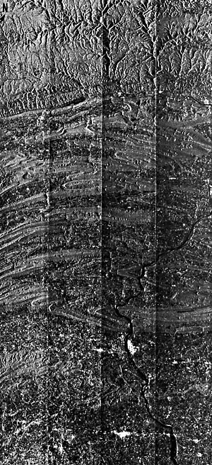 |
|---|
The typical mode of operation and character of signal return for a radar system are depicted in Figure A-6. The outward-sweeping beam scans a strip of surface elongated normal to the azimuthal direction of flight. Its length is set by the depression angle (measured from the horizontal) downrange along the look direction. Its complement, the incidence angle, is measured from the vertical. Photons in the energy burst interact with the ground targets, creating new radiation, some of which is returned to the antenna where it is converted to an amplified electrical signal. The strength of that signal depends on a number of variables, mainly the geometry (shape) of the surface, the physical roughness of the surface relative to the wavelength of the pulse transmitted, and the dielectric constant of each material present in the target area. In the schematic diagram, the sensor-facing slope of the hill sends back considerable energy to the radar receiver, but the opposite slope is not illuminated by the beam, which causes a dark shadow. Plants and other vegetation scatter the radiation from their leafy surfaces, but a moderate amount is returned to the radar. The metal bridge consists of planar surfaces and corners, some oriented to efficiently return a high fraction of the beam. However, water, if not churned up by waves, acts as a specular reflector that redirects the radiation away from the receiver.
If surface roughness (as from pebbles or pits) has average dimensions much different (usually larger) than the radar wavelength, it acts to produce considerable backscatter that results in a strong (bright) signal return; a smooth surface relative to the radar wavelength generates a weak (dark) signal because of significant specular reflection away from the sensor. Likewise, because leaves may or may not interfere with the radar waves, depending on leaf size and on the radar wavelength, some tree canopies can be penetrated. Clouds are "transparent" because cloud-vapor droplets are too small to interact with most radar wavebands. However, ice crystals and raindrops may back scatter a signal. Reflection of radar radiation back to the antenna increases as the relative dielectric constant becomes smaller (3 to 16 for rocks and soils and 80 for pure water); a dry soil or sand (very low dielectric) permits penetration to depths of meters in some cases.
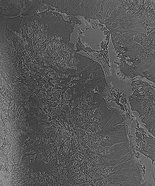
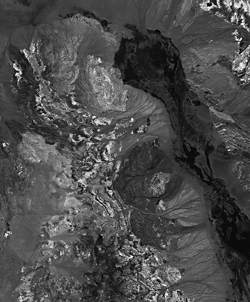
| Figure A.8. Four products of image enhancement of a Landsat-5 Thematic Mapper subscene (50114-17550, June 23, 1984) of the Death Valley, California, area (see Plate T-5): (a) band 3 "raw" product (minimal enhancement), (b) band 3 gaussian stretch, (c) band 3 high-pass filter plus stretch, and (d) band 3/4 ratio. | |
|---|---|
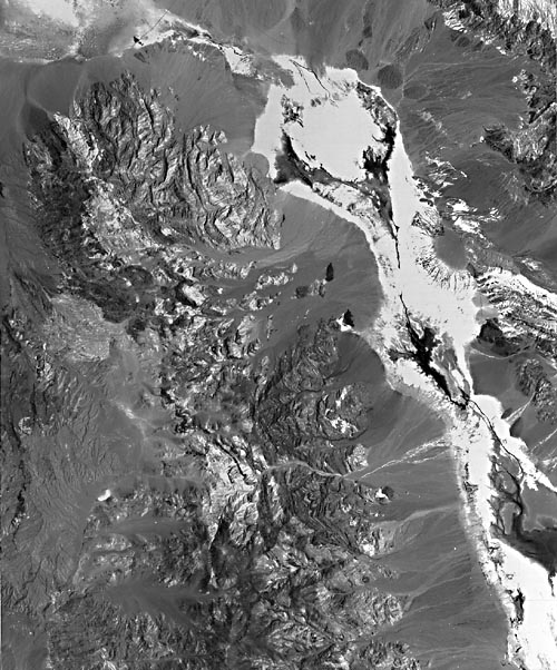 | 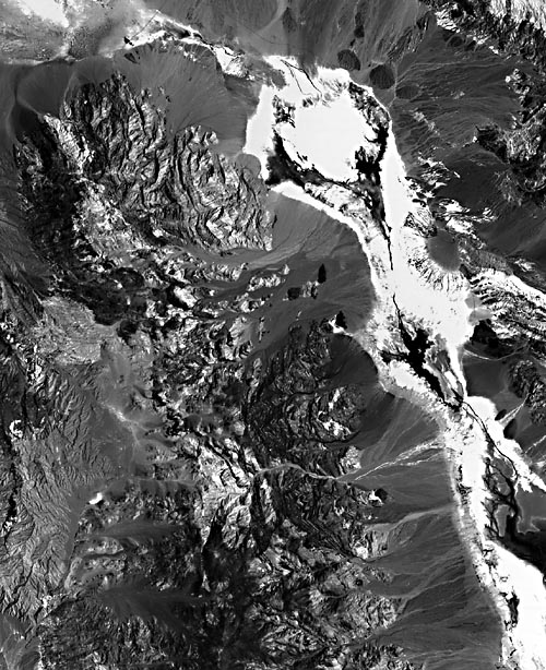 |
 |  |
Radar images can be generated on recording devices from the electrical signals whose magnitudes are proportional to the returned radiation intensities. By convention, strong signal returns are printed as light tones and weak ones as dark tones (Figure A-7). Because of the proximity of airborne radars to the ground (as contrasted to the far greater distance of the Sun to a local surface on Earth), the geometry of radar-sensed features (such as hills) on the ground is more prone to distortions than that in images obtained with natural illumination. Distortions also vary as the depression angle changes from near to far range. Close in, foreshortening is expressed by an imposed asymmetry on forms such as ridges, so that the radar-facing slopes appear to steepen (the bright pattern becomes narrower) and the back slope broadens (dark pattern wider); this effect diminishes with decreasing depression angle. In the extreme, the facing slope appears to "layover" if its foreslope is greater that the look angle.
IMAGE ENHANCEMENT OF GEOMORPHIC SCENES
Many of the space images appearing throughout this book have been subjected to special computer-processing to more sharply define the geomorphic features and other geologic information that led to their selection. Although various techniques and operations can be applied to the data from which these images are constructed (see Condit and Chavez (1979) for a succinct summary of digital image processing or Short (1982) for a more in-depth review), several known collectively as image enhancements are generally the most useful to geomorphologists simply because they tend to improve the spatial display and characteristics of landforms in a scene. These are described briefly in this section, with emphasis on integrating the computer into the enhancement option.
Any experienced photographer is fully aware of the value of imparting an optimal contrast, or levels and spread of tone distribution, to a photograph. This usually involves expanding the number of discernible gray levels; the process is called contrast-stretching. The result is a picture both pleasing to the eye and, in scientific photography, effective in increasing the information content. At one or more stages in the entire photographic process, contrast can be influenced by various factors: at the time of picture-taking, such conditions as film type used, lens filters, illumination, and other exposure variables; in processing and printing, film development conditions, filters, properties of the printing paper, and exposure times.
The printing of a Landsat image is also affected by similar factors, but the importance of the film negative generated from the digital data is often paramount. Superior contrast can be introduced at some stage of negative production by manipulating the range of radiances (usually as reflectance) emanating from the scene and modified by the sensor. These radiances, expressed as digital numbers (DNs), fall within a range defined by gain settings and other sensor characteristics. For a Landsat MSS data set, the levels of brightness that can be detected by the sensor are digitized over a DN range of (2n-1; n = 1 to 8) or 0 to 225. Now, suppose the normally gaussian distribution of DNs representing the radiances from a given scene, after those are quantified and digitized, is 40 to 110. A photographic negative made to image this spread of values might have a limited range of gray levels within a particular film used, depending on the gamma (density transfer function) of the characteristic curve (X-Y plot of density D versus log exposure E) chosen; in other words, the negative may be "flat" and would produce a low-contrast positive print. Using an appropriate program, a computer can systematically expand (or contract, for a scene marked by a wide spread of radiances) the DN range so that a new negative will contain more of the gray levels that potentially are available within the density response capability of the film or print paper. (Of course, the benefits of such a stretch can be reduced by ineffective photo-processing afterward.) "Before" and "after" images following stretch-processing by computer are exemplified in Figures A-8a-b. Various kinds of numerical stretching are possible in computer-based processing, including linear, stepwise linear, logarithmic, and probability distribution function expansions or contractions. Similar principles of stretching underlie the moderation of contrast on electronic image displays (such as a television monitor).
| Figure A.9. Classification of a Landsat-5 Thematic Mapper subscene of the Waterpocket Fold (monocline) between Circle Cliffs and the Henry Mountains (see Plate F-6); classes are stratigraphic formations; training sites selected from several U.S. Geological Survey maps (Short and Marcell, 1985). |
|---|
 |
Another enhancement approach involves combining sequential DNs within a specified range into a single gray level or density. Adjacent DN ranges over the total distribution are treated in like manner, thus reducing the variation of many individual brightness values to a new set of much fewer values. This method, known as density slicing, produces a simplified pattern of varying tones in a black and white image; each composite gray level can likewise be assigned a discrete color to visually enhance the image display by color coding. Sometimes a surface feature, such as a landform type, has a unique or characteristic tonal signature and a narrow range of gray tones, allowing it to be separated as a particular pattern by slicing its mean level and spread from other levels.
A powerful enhancement technique that sharpens an image and can selectively bring out or delineate boundaries is addressed under the general term of spatial filtering. In any X-Y array of brightness values, like that of pixels in an image, the changing value can be considered to vary in a spatial as well as a radiance sense. This spatial variability can be expressed as frequencies (number of cycles of change over a given distance). A low spatial frequency represents gradual changes in the quantity (e.g., DNs) over a large areal extent of contiguous pixels; high spatial frequency results from rapid changes as only a few pixels in an area of the array are traversed. Variable line spacings in resolution test patterns are an artificial example of differing frequencies. (This can also be related to the concept of Modulation Transfer Function (MTF) that is a fundamental property of films or images.) Any image (or a complex harmonic wave) can be separated into discrete spatial frequency components by the mathematical technique known as Fourier Analysis.
Spatial filtering of an image can be done by scanning vidicons equipped with special functions; alternatively, the input data (DNs) from which images are derived after scanning (as by an MSS) are run through algorithm-based "filters" in a computer program designed to screen out or diminish certain frequencies and pass or emphasize other frequencies. To do this, a traveling "window" or "box" consisting of an array of n x m (line and sample) pixels is set up. This, in effect, creates a new value for each pixel as it passes during the computations into the center point of the moving array; the new DN for each such pixel depends on the brightness value frequency distribution of its neighboring pixels in the array size chosen. A low-pass filter ("band-pass" when the image data come from a spectral interval or band) tends to respond to features (including separated natural landforms such as dunes, divides, streams, fracture-controlled lakes, and series of folds) whose sizes and recurrence intervals (spacing) are larger than the averaging array (i.e., high-frequency spacings are not picked up). A high-pass filter reacts to features having dimensions and spacings smaller than the array. The new set of pixel values resulting from this will enhance (sharpen) those features whose periodicity or scale allows them to be enhanced. This filtered data set can be converted directly into a new image or can be combined (restored) with another image (such as the original one with its particular tonal patterns). The new image is usually contrast-stretched in the process to bring out density differences among the pixels in the array. Linear features such as rock or stratigraphic contacts and lineaments thus emphasized are said to be edge-enhanced. An example from the spatial filtering process is presented in Figure A-8c.
Although not an enhancement process in the strict sense, the ratioing of brightness values in one spectral band to those of equivalent pixels in another band yields a new set of DNs from which another image can be generated (Figure A-8d). For MSS data, this allows comparisons of relative reflectance between spectral intervals. Consider a ratio of bands A to B: a high value for A reflectance and a low for B produces a high ratio whose DNs would give rise to light-gray tones; conversely, low A and high B values cause low ratios and dark tones; similar A and B values lead to intermediate tones. Three sets of ratio images (e.g., A/B, C/A, D/B) can be combined into color composites with various colors often diagnostic of particular materials.
Identification of objects or features and materials by one of several methods of computer-directed classification can be treated as another means of the information extraction that is the ultimate goal of enhancement. The essence of the concept underlying classification is this: each identifiable class of object/material is considered to have one or more distinguishing properties with certain statistical parameters (usually means and variances) that can be demonstrated to be different (statistically) for other classes set up or recognizable in the data set being analyzed (such as natural terrains or land cover on a planetary surface). The classification program clusters property data into separable numerical sets (unsupervised classification) or obtains data characteristic of each known class in the scene by sampling those data at specific training sites (supervised classification). Once the specific classes are established from a fraction of the total sample points (e.g., pixels in an image), then all other (still unknown) sample points are assigned to some given class, identified by comparing their parametric characteristics (within the bounds of the statistical limits chosen) to those of the classes defined initially. Each unknown point is thus matched up with the class whose selected property or properties (e.g., radiance in an MSS image) is stochastically closest to it.
Classification of a Landsat image is usually based on spectral properties. An example of a geologic scene classified into rock/stratigraphic units by sampling the reflectance of each recognizable formation appears in Figure A-9. Other classifications can be devised to include spatial information (pattern recognition); although this has seldom been done yet for the geomorphic content of space imagery, in principle, it could be readily accomplished.
CLOSING REMARK
This necessarily brief exposition of the principles of remote sensing was designed to introduce those unfamiliar with interpreting sensor-created images to those main ideas needed to appreciate the varieties of space and aircraft multispectral, thermal, and radar images appearing throughout this book. For a fuller understanding, consult any of the references cited in the introductory paragraph of this Appendix.