Introduction

Principal Components Analysis is a procedure for transforming a set of correlated variables into a new set of uncorrelated variables. This transformation is a rotation of the original axes to new orientations that are orthogonal to each other and therefore there is no correlation between variables. The graph below shows a plot of band 2 versus band 1 of the Morro Bay TM scene. As you an see, the value of band 2 for a particular pixel is related to the value for band 1. The correlation is high.

Since the rotation is a linear combination of the original measurements, if all of the axes are included in the rotation, no information is lost. "No information is lost" means that the original measurements can be recovered from the principal components. If the original data set is singular, then principal components will produce a new representation that is not singular. There are several ways of viewing this transformation:

1. It can be viewed as a rotation of the existing axes to new positions in the space defined by the original variables. In this new rotation, there will be no correlation between the new variables defined by the rotation. The first new variable contains the maximum amount of variation, the second new variable contains the maximum amount of variation unexplained by the first and orthogonal to the first, etc...

2. It can be viewed as finding a projection of the observations onto orthogonal axes contained in the space defined by the original variables. The criteria being that the first axis "contains" the maximum amount of variation, or "accounts" for the maximum amount of variation. The second axis contains the maximum amount of variation orthogonal to the first. The third axis contains the maximum amount of variation orthogonal to the first and second axis and so on until one has the last new axis which is the last amount of variation left. As you can see these are really two slightly different ways of saying the same thing!

There are several algorithms for calculating the Principal Components. Given the same starting data they will produce the same results with the one exception (are you surprised?). This exception is that, if at some point, there are two or more possible rotations that contain the same "maximum" variation, then which one is used is indeterminate. In two dimensions the data cloud would look like a circle, instead of an ellipse. In a circle, any rotation would be equivalent. In an elliptical data cloud, the first component would be parallel to the major axis of the ellipse.

To calculate the rotation we can start with either a Variance-covariance Matrix or a Correlation Matrix. If one standardizes the data and calculates a Variance-covariance Matrix, then the result will be the same as a Correlation Matrix. Those that wish to practice their algebra can prove this by deriving the formula for the Variance-covariance Matrix and the Correlation Matrix calculated on "raw" data and then the Variance-covariance Matrix calculated on standardized data.

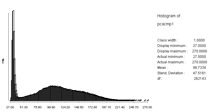
The histogram of the first Principal Component for the Morro Bay scene is:

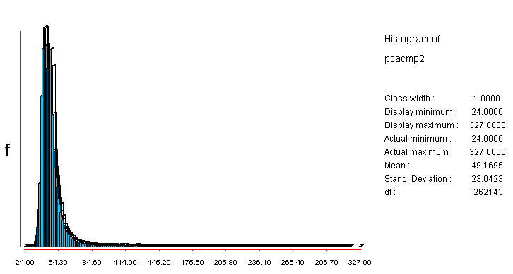
The histogram for the second Principal Component of the Morro Bay scene is:

Compare these with the histograms of the original bands.

We can plot the second principal component versus the first to get the 2D view that follows.

How do we get this figure? The elliptical cloud that lies parallel to the X axis is what we might expect. But we need to remember is that we are carrying out our rigid rotation of axes in a 7 dimensional space, one for each band (or variable). We can see here that the original data was not Multivariate Normal, an assumption that would need to be met if one wanted to carry out any parametric statistical tests. This non-normality is indicated the anomalous cloud of points going diagonally across the graph. If the data were multivariate normal in 7 dimensions, then the plot would only have a cloud like the horizontal one in the above plot.