Remote Sensing Tutorial Page 1-13

Another processing procedure that often divulges valuable information of a different nature is spatial filtering. Although less commonly performed, this technique explores the distribution of pixels of varying brightness over an image and, especially detects and sharpens boundary discontinuities. These changes in scene illumination, which are typically gradual rather than abrupt, produce a relation that we express quantitatively as "spatial frequencies". The spatial frequency is defined as the number of cycles of change in image DN values per unit distance (e.g., 10 cycles/mm) along a particular direction in the image. An image with only one spatial frequency consists of equally spaced stripes (raster lines). For instance, a blank TV screen with the set turned on, has horizontal stripes. This situation corresponds to zero frequency in the horizontal direction and a high spatial frequency in the vertical.

In general, images of practical interest consist of several dominant spatial frequencies. Fine detail in an image involves a larger number of changes per unit distance than the gross image features. The mathematical technique for separating an image into its various spatial frequency components is called Fourier Analysis. After an image is separated into its components (done as a "Fourier Transform"), it is possible to emphasize certain groups (or "bands") of frequencies relative to others and recombine the spatial frequencies into an enhanced image. Algorithms for this purpose are called "filters" because they suppress (de-emphasize) certain frequencies and pass (emphasize) others. Filters that pass high frequencies and, hence, emphasize fine detail and edges, are called highpass filters. Lowpass filters, which suppress high frequencies, are useful in smoothing an image, and may reduce or eliminate "salt and pepper" noise.

Convolution filtering is a common mathematical method of implementing spatial filters. In this, each pixel value is replaced by the average over a square area centered on that pixel. Square sizes typically are 3 x 3, 5 x 5, or 9 x 9 pixels but other values are acceptable. As applied in lowpass filtering, this tends to reduce deviations from local averages and thus smoothes the image. The difference between the input image and the lowpass image is the highpass-filtered output. Generally, spatially filtered images must be contrast stretched to use the full range of image display. Nevertheless, filtered images tend to appear flat.

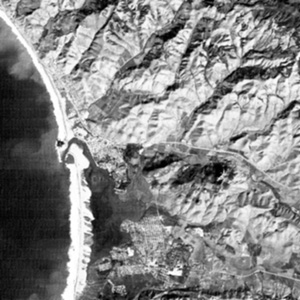
Next, we will apply three types of filters to TM Band 2 from Morro Bay. The first that we display is a lowpass (mean) filter product, which tends to generalize the image:

An edge enhancement filter highlights abrupt discontinuities, such as rock joints and faults, field boundaries, and street patterns:

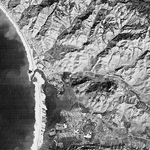
In this example, the scene retains its general appearance but it highlights streets and some ridges are better defined. Note, too, the sediment boundaries are easier to see.

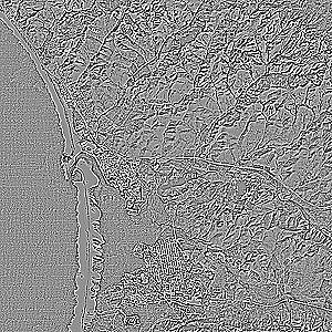
Here, streets and highways, and some streams and ridges, are greatly emphasized. The trademark of a highpass filter image is that linear features commonly appear as bright lines with a dark border. Details in the water are mostly lost. Much of the image is flat.

1-13: Comment further (evaluate) the three filter images shown above in terms of what information you extract visually. Include detrimental aspects. ANSWER

Webmaster: Bill Dickinson Jr.
Site Curator: Nannette Fekete
Please direct any comments to rstweb@gst.com.

Spatial Filtering