We can measure heights of surface features (e.g., tall trees and buildings) and relief by various photogrammetric techniques. Consider for example, determining the height, h, of a tall building that lies near the edge of a single aerial photograph. If that photo was taken vertically, i.e., looking straight down, then its center lies at the nadir (the vertical line from camera perpendicular to a surface point directly beneath [assumed to be flat ]). In that instance, the nadir coincides with the principal point (p.p.) in the photo, which is the intersection of the lens' optical axis (as though extended) and the ground, so that the p.p. is also the true center of the photo. That point becomes off-center, if the photo (and optical axis) is non-vertical. If the building were to lie close to the p.p., its top and bottom would appear to coincide in the photo. If it is well away from that point at some radial distance, r, towards the edge, its viewed state at a slant would have the top displaced further away from the p.p. than the bottom by some amount measurable in the photo as, d. For an aircraft height, H, (calculable from the scale if we know a ground distance), the value of h is just, h = (d/r) x (H). We can illustrate this approach with a large scale, low camera altitude aerial photo of the downtown area of Long Beach, California (from Sabins, 1987; courtesy J. Van Eden), in which the lateral tilt of tall buildings is obvious in the outer parts. Here, we drew d and r between the p.p. and one of the buildings near the edge:

11-11: Using this figure, determine the height h of the building to which are drawn white arrows to distances d (photo displacement from bottom to top) and r (to building top). On the actual photo (not your screen) d = 0.5 inch and r = 3.0 inches. Scale of the photo is 1:3600. Aircraft altitude is 1800 ft. ANSWER

We can calculate height differences (relief) between points of different elevation along surfaces from stereo pairs using this formula, h = (H) dP/(P + dP). Cross-check the figure above and the drawing below as an aid to visualizing the process. We show the two photos in the drawing cockeyed, typical of the effects of inflight yawing (rotation around a vertical axis).

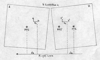
Parallax (defined on page 11-3) is actually a physical condition that refers to the displacement of a point or a feature of some height in an photo or image caused by a shift in the position of observation. This will occur in aerial or space photos that have been taken in succession (such that a stereo pair has either overlap (same flight line) or sidelap (parallel flight lines). P is the absolute stereo parallax. For any standing object or separated points on a slope whose height or relief we want to determine, we measure the distance (in the direction parallel to the flight line) on one photo between the base (here, point b) of that feature and the principal point (PP1) or nadir. We then do the same for that conjugate feature as it appears in a different position in the other photo. Note that the first photo p.p.(pp1), now lies at some distance off-center (at pp1') from the second photo p.p. (pp2). Then we average the two distances (d1 + d2 divided by 2).

The dP term is the differential parallax. We find it by measuring the distance between the base and the top of the feature or between two proximate terrain points at different elevations on a slope, that we locate in each of the two photos when the pair is in optimum alignment for stereo viewing. Then, dP is the numerical difference between the two distance values (x₂ - x₁), which is different in each of the photo pairs. We can optically find the value of dP by using special devices, such as a stereometer, a parallax wedge, or, most commonly, a parallax bar. Each uses a variant of the "floating point" method in which reference marks–dots or crosses–are visible when we view the aligned photos under a mirror stereoscope. We place the parallax bar on the photo plane so that a fixed mark over one photo coincides with a movable mark (fused visibly in the stereo view) by turning a screw drive that translates that mark into coincidence. We then read the value of dP from a graduated scale. When we do this for a number of points, then, we can calculate heights and relief values for parts of the map. These become absolute values (elevations), if we reference the points to benchmarks.

11-12: A stereo pair was obtained from a photo mission flown at 2000 meters. We wish to determine the height of a water tower (storage tank on legs).The photo base length P between the two photos when properly placed for effective stereo viewing is 70 mm. The differential parallax dP for the tower, as measured by a stereometer, is 0.4 mm. What is the height? ANSWER

Using the above devices to specify a large enough number of elevation points in stereo photos to permit contouring is difficult and tedious. Instead, we apply sophisticated optical-mechanical stereoplotters. These devices use two or three movable projectors that pass light through stereo pairs made into glass-mounted film diapositives placed onto a tracing table (platen) which we can raise and lower. We produce a 3-D image or stereomodel, which an outside observer can view by some filter method. For black and white photos, we do this by the anaglyph method, in which we project one photo through a red filter and the other a cyan filter and then view them through eyeglasses with corresponding color filters. We project a small point of light or dot onto the stereomodel. When the dot appears to coincide with some part of the model surface (as seen through the viewer), that dot locates a particular elevation determined by the platen height and calibrated by control points. An experienced operator can then move the light along the model surface, such that it always remains coincident. This motion traces a contour line. They then raise (or lower) the platen table a fixed amount determined by the chosen contour interval and they contour the next elevation. This process continues until they trace the entire surface. Today, analytical stereoplotters are capable of semi-automating the contouring through computer processing of mathematically transformed data.

In recent years, contour values have been digitized allowing us to manipulate them into versatile displays of topographic data as digital elevation models or DEMs. Digital terrain models (DTMs) are variants that show additional landscape attributes. We can use existing maps as inputs by tracing contour lines on a digitizing tablet or table. The data are organized into cell arrays whose X-Y positions in the rectangular grid are related to map coordinates. Each cell has a single value representing the average elevation of the land surface within it. The finest-sized cells are 30 meters on a side, associated with the 7.5 minute topographic quadrangles mapped by the USGS using the Universal Transverse Mercator (UTM) coordinate system. Only a fraction of the maps at this scale have been digitized, as yet. This digitizing is also true for 15 and 30 minute maps. To date, all of the 50 U.S. states, except parts of Alaska, mapped at 1:250,000 scale (extending over 1 degree by 1 degree in eastern states and 1 degree by 2 degrees in western states) have now been digitized at a cell size of three arc seconds. They store the data in east-west profiles.

You can access a general review of the concepts and mechanics of producing DEMs at a site maintained by the Eros Data Center (EDC). http://edcwww.cr.usgs.gov/glis/hyper/guide/usgs_dem

Collaborators: Code 935 NASA GSFC, GST, USAF Academy
Contributor Information
Last Updated: September '99

Webmaster: Bill Dickinson Jr.
Site Curator: Nannette Fekete
Please direct any comments to rstweb@gst.com.