So far, the spectral plots displayed on the preceding page are mostly pure phases, irradiated under laboratory conditions. Even under ideal conditions, though, for the same species, notable physical and/or chemical variations can exist, e.g., ones related to color or from foreign coatings (such as iron rust). So, a single spectrum, while containing the dominant and diagnostic absorption features for a species, is a standard that we must generalize. Straightforward chemical changes can significantly modify the spectrum. Many minerals, for example, allow substitutions of one element or ion state at lattice sites by other elements, so that the formula for such materials is variable. Take, for instance, the progressive substitution of aluminum in certain octahedral sites that occurs in the common mica, Muscovite. Note how this affects the principal absorption trough at 2.2 µm. Again, the curves are offset.

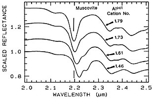
13-24: Devise a rule for the shift of a diagnostic absorption band with increasing amounts of Aluminum substitution. ANSWER

The size range of individual mineral grains or crystals can have a major effect on the characteristic spectral curve of the same species. This usually influences the total reflectance but can also modify the depth of an individual absorption feature. Consider the effect of grain size (in µm) for finely ground samples of the same specimen of a pyroxene species (there is no offset applied to these curves).

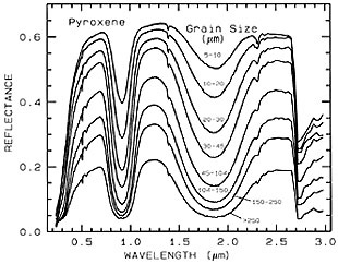
As the grain size enlarges, the reflectance diminishes, although the absorption troughs remain relatively constant. Two factors control this effect: the larger grains allow more absorption and the smaller grains provide a higher proportion of surface area available as reflectors.

13-25: Explain the effects of grain size change on the spectral curves. ANSWER

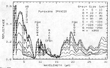
Rather unexpectantly, there is a broad reversal in the relative reflectance as a function of grain size when we examine the same material in the mid-IR region, as shown here:

As we saw earlier in this section, mixed pixels are the rule for most space images and become ever more troublesome as resolution increases. This problem can be even greater when we acquire a single spectral curve for the features and classes normally present in a pixel, representing Landsat Multispectral Scanner or Thematic Mapper resolutions. The resulting spectral plot shows a variety of absorption troughs, some of which we can match to individual phases (classes), whereas others may lie in nearly the same wavelength positions, but are really other bands that are present in common with the phases. The reflectance at any given wavelength is also a composite average of the proportionalized phases contributing to the mixture.

To illustrate this for two simple cases, observe these curves. The first is just a series of a two-phase mix, in which the clay mineral Montmorillonite is progressively diluted with charcoal, which has a spectral curve with no absorption troughs and an overall low reflectance.

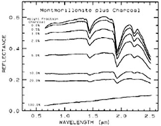
The reflectances are absolute (no offsets). The result of adding the black charcoal to the whitish Montmorillonite is to reduce the depths of the absorption troughs. Above 20% charcoal, the toughs nearly disappear due to the dominance of charcoal in reducing reflectance.

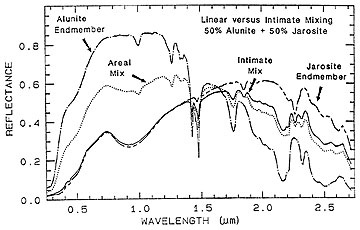
Now look what happens when we mix two very similar minerals, Alunite (a potassium sulphate also containing aluminum) and Jarosite (the same, except iron replaces the aluminum) in two different ways: Areal, which we compute as a linearly equal combination of the two end members, and Intimate,which we combine and thoroughly intermix and then irradiate under laboratory conditions. The darker (yellow-brown) Jarosite has a lower reflectance continuum at the shorter wavelengths but becomes higher at longer wavelengths. In a 50-50 mix, this darker phase predominates, so that the reflectances are (similar to the effect of charcoal) controlled almost entirely by Jarosite.

From the above considerations, we learn that practical remote sensing, which depends upon imaging spectrometers and hyperspectral data acquisition is especially sensitive to many variables, including foremost, the mixed pixel problem. Because the spectral curves that we can derive from sensors, such as AVIRIS. vary "all over the place," from pixel to pixel, as the combinations of surface features change in a scene, we need some method(s) of reducing the data to meaningful components that we can assign to their proper classes. We must simplify complex spectra, containing contributions from a variety of phases (in a single 30 meter square pixel soil, water, vegetation, buildings, etc. can mutually occur), so that we can extract the identity and proportions of each. Fortunately, with effective mathematical models and computer processing, we can do this task with surprising effectiveness.

This subject of hyperspectral data reduction and analysis is specialized and somewhat complicated, so that we offer only an outline of the approaches used.

The starting point (and the key) is to develop a Spectral Library. This library consists of literally thousands of individual spectral curves, obtained by spectrometers applied to discrete materials (as pure as possible,) and classes in laboratory and field settings. This library has built up over the years as a data collection developed from many observations by numerous groups. Best known in the U.S. is the library assembled by the Spectroscopy Lab of the U.S Geological Survey in Denver. (For more information, check their Home Page).

From such information, spectralÐfeature, identification algorithms have been devised to quantitatively analyze hyperspectral data, acquired during aircraft overflights. The U.S.G.S. has put together such a program known as Tetracorder, which contains various routines that systematically reduce the raw data to specific identifications. It convolves individual fits of library curves to the hyperspectral data obtained from a mission. In some instances, it can analyze a complex (composite) curve by appropriate algorithms that break it into a set of "end member" curves, each representing a material or class that is a component of the curve. It calculates band locations (indexed to the wavelength at the bottom of the trough) and depths, using a continuum base as reference. The weighted fit leads to correlation coefficients that a least squares routine numerically fixes. Band ratios can also prove helpful

Since spectral bandwidths may be broad, analysis of many individual channels (for AVIRIS, 224 spread continuously from 0.38 to 2.5 µm) is customary. However, an analysis need not sample all the channels for certain problems. If the task is to identify a group of minerals in an alteration zone in a mining district, located in a vegetation-sparse region, the critical interval between 2.1 and 2.5 µm containing enough diagnostic absorption bands may suffice to identify them. For some identifications, data from two, three, or a few more channels may be sufficient to identify a particular class in compositional detail. Examine this plot that shows variations in a band-bottom, point wavelength as a function of compositional variations in pyroxene minerals, present in an area undergoing mineral analysis.

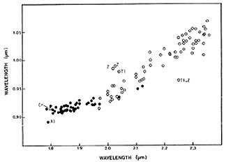
From such data, we devise correlation coefficients relating composition to wavelength using least-squares statistics.

Of course, it is usually not expedient to plot spectral curves for every pixel in a mission data set. Instead, the spectral data serve to pinpoint the individual materials present in the pixel and then we can display the results in a map or image-the usual display type in presenting the results of a scene analysis. If the spectral resolution is high (a few meters), then commonly we assign a dominant class to each pixel. In the real world that we want to picture, that dominant class may extend over many pixels, leading to a hyperspectral image that has similar characteristics to typical Landsat scenes. But, the ability to fine-tune the class identities, and to record separately some of the nature of the mix, are the great advantages that emerged with imaging spectroscopy, as a significant improvement in sensor technology for remote sensing.

Collaborators: Code 935 NASA GSFC, GST, USAF Academy
Contributor Information
Last Updated: September '99

Webmaster: Bill Dickinson Jr.
Site Curator: Nannette Fekete
Please direct any comments to rstweb@gst.com.