Remote Sensing Tutorial Page 17-7

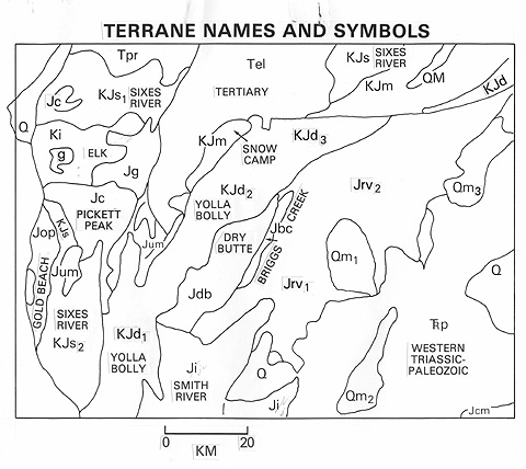
For the writer's research project, he selected a segment of the Oregon Klamath Mountains for prime attention, although for some tasks he also looked at adjacent areas. The following map displays the area, on which he drew terrane boundaries, named the terranes, and assigned stratigraphic symbols to each (the first letter(s) denote(s) their ages in terms of geologic periods, with Tr = Triassic; J = Jurassic; K = Cretaceous; Tel = Tertiary; Q = Quaternary). He digitized the boundaries on the map to allow "cookie-cutting" of geographic data in other maps, so that he could group the data into categories for terrane analysis.

By comparing the above terranes map with the geologic-units map for all of western Oregon (below), we see a close correspondence

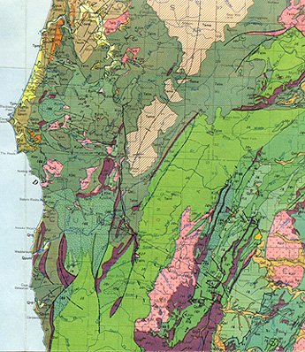
between some units and their enclosing terranes, a broader correspondence for others, a number of individual units that are scattered about within the terranes, and some units that seem to cross over or overlap terrain boundaries. Because there are so many units [generally, at the formation level], we don't show the map's legend. Also, in the legend sequence are units that aren't present in the Klamaths. Two examples of exceptions are the deep purple unit (Jui), which is actually outliers of ultramafic (ophiolitic) lavas, once part of oceanic crust, which appear similar in the field but originated locally within their terranes, and the pinkish-red unit, which consists of intrusive rocks that invaded several terranes, already in place. We expect this general agreement between terranes and their constituent stratigraphic units (i.e., internal consistency), along with the exclusivity of some units to single terranes, inasmuch as terranes typically develop from rocks formed in different source areas at different times.

17-17: Although it will require considerable scrolling up and down on this page, go ahead and try to match the different color units in the geologic map with the terrane units in the map above. ANSWER

The Oregon Klamaths are among the most rugged landforms units in the state. We can gain a sense of their appearance by inspecting this 3-D perspective image of nearly all of Oregon, generated from DEM data:

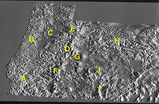
Features of interest in this shaded map are: A = Klamath Mountains.; B = Coast Ranges; C = Willamette Valley (Portland at the north end); D = High Cascades; E = Mount Hood; F = Crater Lake; G = Paulina Mountains (Newberry Crater); H = Blue Mountains.; I = Abert Rim; J = Summer Lake area (the circular area is somewhat an artifact of the illumination)

We get a feel for the appearance from the ground of several of the Klamath terranes through these photographs taken during the writer's time in the field:

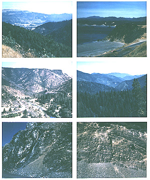
The upper left scene shows terrain around Canyonville, with Yolla Bolly terrane in the foreground and Sixes River terrane in the distance. Next to it is a view from the coast of the Elk terrane. In left center is a segment of a canyon dissected by the Rogue River, in which sedimentary units of the Rogue Valley terrane (Jrv) are exposed. To its right is landscape typical of the higher elevations in the Klamath Mountains. The lower left scene is an exposure of serpentinite (the metamorphosed ophiolitic basalts associated with oceanic crust). The lower right shows alternating layers of siliceous (cherty) shales that constitute island arc sediments. Here they are part of the Yolla Bolly terrane.

We afford a preview of the topographic expression of the Klamath Mountains, which we will present from Landsat shortly, by this enlargement of the area made from the same DEM data. Notice Crater Lake (nearly circular on top of a mountain) in the upper right part.

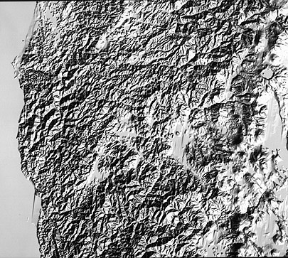
The terrane map is reproduced here again to aid you in matching units to their DEM expression. Keep in mind that the DEM version covers a notably wider area.

In this visual version, we have trouble seeing any significant variations in terrain that call attention to noticeable terrane differences. Of course, we can vary the illumination directions to emphasize contrasted ridge and valley orientations, We did vary the illumination directions on this data set, giving several distinct expressions but, again, obvious patterns that correlate with the various terranes as mapped did not stand forth. However, when we learn where to look, after familiarization with terrane locations, strong hints of certain differences for several of the terranes are discernible. We can also disclose these differences by appropriate analysis of topographic data in map-sheet or DEM formats and, in fact, this approach proved superior to visual differentiation.

The reason we would postulate for expected differences is that each terrane consists of a group of rock types that will likely differ from other nearby terranes. Fault discontinuities also bound each one, at least partly. A terrane will respond to regional erosive action according to its mix of lithologies. Thus, any one terrane may develop landform characteristics that differ from its neighbors and can appear visually as separable. We should be cautious about expecting the differences to remain neatly within terrane boundaries, because, as the landscape develops within any one terrane, the equilibrium forms tend to exert some influence on terrains outside the boundary. Nevertheless, the hope in testing the hypothesis of distinctive terrane-controlled topographic expression is that real differences do occur.

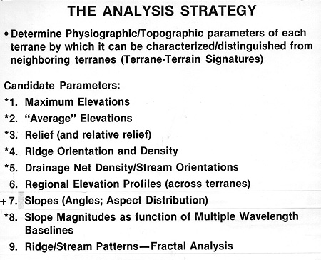
We predicate this effort on making a series of quantitative measurements that we could test numerically and statistically to ascertain valid differences in the topographic character of each terrane. In general, we can't extract any of these measures with confidence from Landsat imagery. However, one SPOT image pair was available, so that we got a stereo image, allowing limited recovery of measurable variables. So, in the exposition that follows, Landsat's prime role is to help to confirm the terrane-terrain association by visual recognition.

Webmaster: Bill Dickinson Jr.
Site Curator: Nannette Fekete
Please direct any comments to rstweb@gst.com.