This is your prime exam in this Tutorial, although subsequent sections will have a fair number of questions of their own. What is different from earlier questions is that most here will be associated with images and maps included in this special subsection, which was drawn from the writer's (NMS) 1982 Landsat Tutorial Workbook. They all relate to a single regional scene that includes much of south-central Pennsylvania and in several images small parts of Delaware and Maryland. Most images are made by the Landsat MSS (remember, Band 4 = green part of the spectrum; Band 5 = red part; and 6 and 7 = Near Infrared). Two thermal and two radar images, made by other sensor systems, are used as well. Some of the image products are computer-derived outputs such as spatial filtered images and classifications.
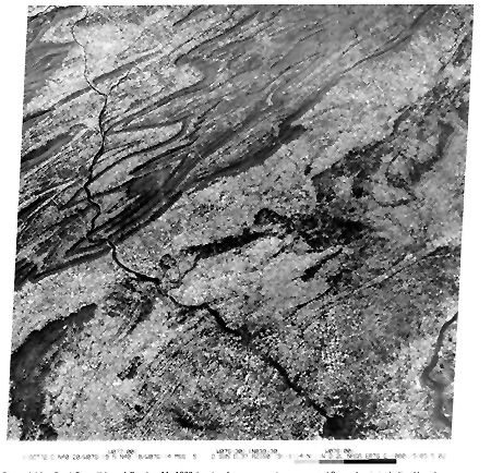
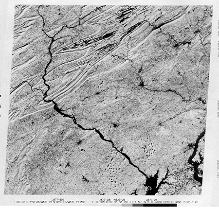
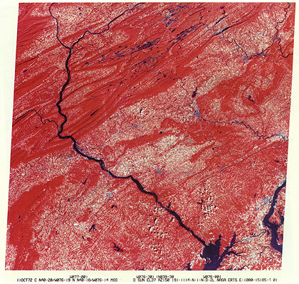
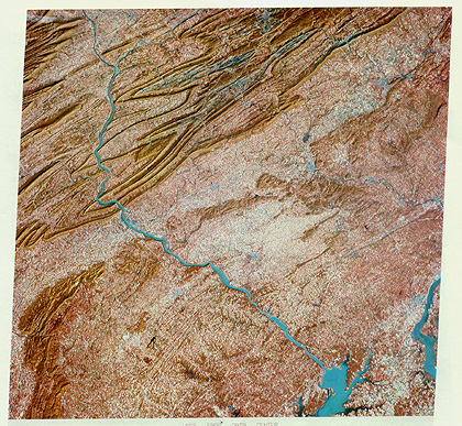
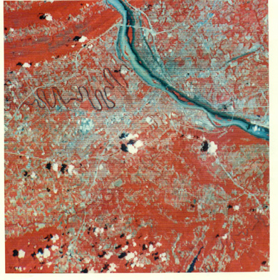
We begin by showing first an MSS 5 image, reproduced on your screen at a nearly 1:1,000,000 scale - the standard size in images distributed by NASA and other agencies and sold commercially. Below it is the corresponding MSS 7 image. And beneath that is a false color composite of the same scene. All were acquired on October 11, 1972 a day after a major storm had hit much of the northeast as far south as southern Virginia. After the sky cleared, the air was especially crisp and dry, cutting down the scene-degrading effects of moisture.
1-1: Using all three images, but especially the Band
7 image, with the help of an atlas or AAA Road Map, locate the following towns
and other features: Harrisburg, York, Gettysburg, Lancaster, Hershey, Lebanon,
Reading, Allentown, Easton, Wilmington, DE, the Susquehanna River, the Delaware
River; the Juniata River. Also, look hard for the small (15000+) town, Bloomsburg,
PA ,which is the current home of the writer (NMS), where this question is being
written. ANSWER
1-2: What other towns, rivers, or natural features
and points of interest in this scene can you list? ANSWER
1-3: How well can you spot the towns and features
in each of the images? What is MSS 5 especially good at bringing to your attention.
ANSWER
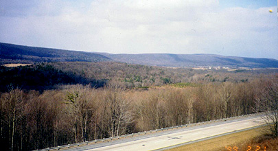
To give you a feel for the typical appearance of the mountain ridges portion of the image, glance at this ground photo taken about 15 km (10 miles) north of the Blue Mountain - the first major ridge encountered going north from the Lebanon Valley. The area photographed, on a February 1999 day when the trees are bare, is along Interstate 81 and lies near the center of the Landsat image.
Now, look at the black and white print of the geological map below that covers most of this scene, plus some surrounding areas.
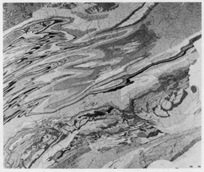
1-4: Fit the major rock unit patterns to the Band
5 image. Comment on the fit. ANSWER
1-5: Comment on what may be unusual about (the color
in) the false color composite. ANSWER
1-6: You may have noted that there is a strip of notation
at the bottom of both the individual band images and the false color composite.
This is on nearly all renditions of Landsat images regardless of the printed
size. We will reproduce this strip, enlarged a bit, just below. Make an educated
guess as to what the different groupings of letters/numbers mean. ANSWER
![]()
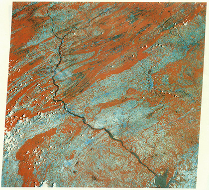
Next, familiarize yourself with this October 23, 1975 false color composite of the same area.
1-7: What overall is different and why? Account for
the blue in the Susquehanna River. ANSWER
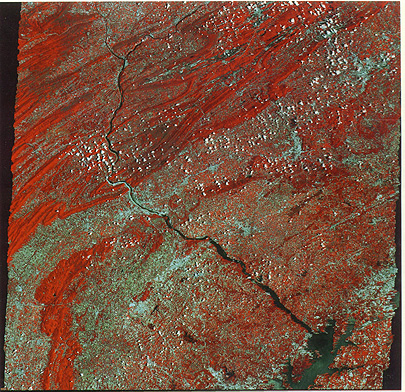
1-8: Now examine the full MSS fcc image of this region
as seen on June 8, 1977. Account for the large areas in blue. Take note of the
dark grayish-black patches on some of the ridges; there are also some blackish
area in the valleys between ridges, primarily in the upper third of the image.
We will take note of these special features later in this exam. Note the course
of the Susquehanna River in the lower third of the image. At several places
the river widens noticeably. Can you explain this. ANSWER
1-9: Below is a scene taken on July 14, 1977. Describe the principal difference between this and the June 8th image. Look also in the vicinity of Harrisburg at the Susquehanna River. It is marked by a blue color on its left side; why? ANSWER
1-10: A Landsat 2 MSS Band 5 scene, taken on January 23, 1979, is reproduced below. Comment on differences you note in this image from those we've examined before. How might one distinguish snow from clouds? ANSWER
At this point, we will zero in on a single localized region, around Harrisburg, to get a better feel for the detail that can be picked out in Landsat MSS imagery (would be much sharper for Landsat TM images with better than 2 _ times higher resolution but a TM image was not available to the writer).
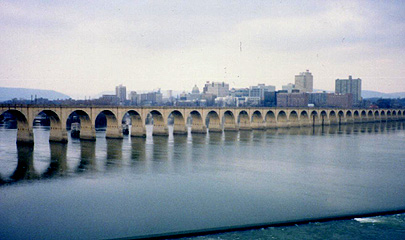
But first, to get up close and personal, look at this ground scene taken from the I-83 bridge looking northeast at downtown Harrisburg. The bridge carries a railroad track across the Susquehanna River. At the far left skyline is a part of Blue Mountain and the water gap through which the river flows
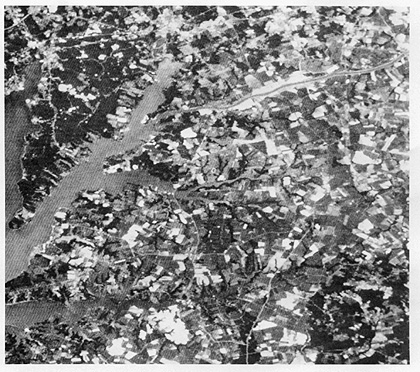
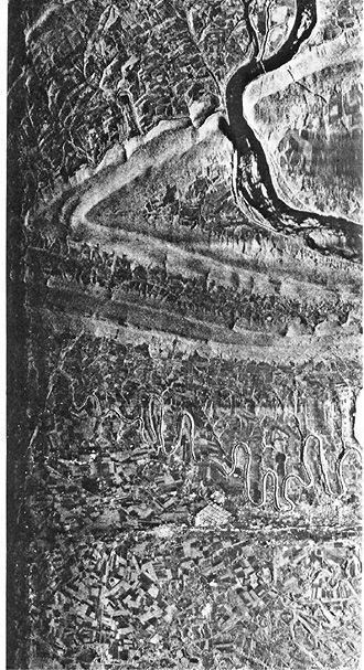
We start our survey from above with a false color aerial photo (scale 1:142,000) taken from an altitude of 50000 feet by a camera mounted on an RB-57's lower bay, on February 5, 1974.
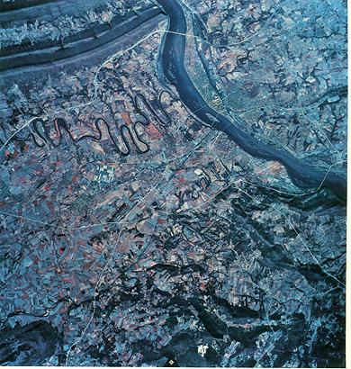
1-11: Peruse this image. Locate Harrisburg first,
then using an atlas pinpoint other towns, major roadways, and the meandering
(curving) river. Mention anything else you find interesting. ANSWER
1-12: Knowing that the standard Landsat full scene
(7.25 inches wide at its base, representing 115 miles across) has a scale of
1:1,000,000, calculate the width in miles of this aerial photo scene. ANSWER
Just below is a subscene from the October 11, 1972 Landsat MSS false color composite which was enlarged to about the same scale as the RB-57 scene above. It was made more blue to look more like
the aerial photo.
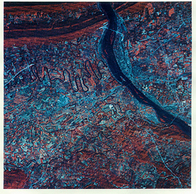
1-13: Compare this subscene with the RB-57 photo,
noting what can be found in both and what is not "seeable" in the Landsat version.
ANSWER
Still another Harrisburg subscene is this July 1977 false color composite.
1-14: Comment on anything unusual or different. ANSWER
We will now look closer at details present in enlargements, concentrating on the area around the Chesapeake & Delaware Canal, south of Elkton, MD. (This is at the lower right corner of the October 1972 scene. The first of two images below is a 512 x 512 pixel subscene from Band 5 of the July 1977
image set. Beneath it is an aerial photo, at a scale of 1:60,000 that contains farmlands included in the Landsat image; this was taken in May of the same year.
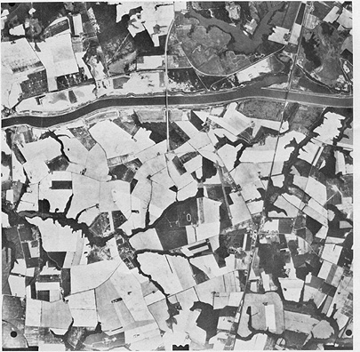
1-15: Can you locate the aerial photo in the Landsat
subscene? Watch out - the field patterns have changed between the two dates
for an obvious reason. ANSWER
We are ready to change directions to concentrate on a prime use of imagery of photo-like nature: change detection. We are going to utilize several subscenes that have been cut from the upper half of the full
images we have already encountered. Consider this first: A June 8, 1977 Band 7 image
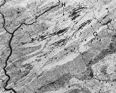
1-16: One thing that is obvious: widespread patches
of almost black features, found almost entirely in valleys between ridges. Do
you have any idea what these represent? Hint: they are related to a geological
material that has immense commercial value; this material is in beds in rocks
of Pennsylvanian age. ANSWER
1-17: There are dark patterns, one elongate, the
other as three spots, near the tips of arrows G and H. What do you think these
are? Can you find them in corresponding local areas in the October 1972 MSS
Band 7 image? What's going on? ANSWER
Now, inspect the scene below which is a July 8, 1973 MSS 7 subscene of the same area just looked at.
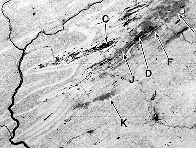
1-18: What's new and different? Identify the features
at arrow tips of the letters indicated (the rightmost arrow is labelled "I").
Features such as at "K" are a new phenomenon, in which the ground is responsible
for the reflectance that gives rise to a medium gray tone (that's a clue!) ANSWER
Pennsylvania was hard hit by the phenomenon at "K" again in 1977. The next illustration is a set of
six subscene panels taken from an area north of Williamsport, PA (just outside the full scenes we have
been looking at). For now, don't read the black print between the two panel rows.
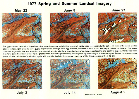
1-19: Since you now know what "K" is from the previous
question, comment on the progression of the feature that appears gray-brown
in these panels. ANSWER
We will now transition into a second phase of questioning in which you will be asked to analyze and
comment on some computer-generated imagery produced in this study of south-central Pennsylvania.
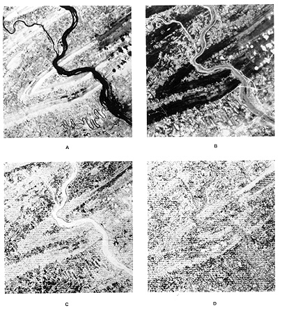
First, is a panel of four subscenes of an area that includes Hanover, PA (at
the left edge, west of the reservoir) about 20 miles south-southwest of York,
PA. Passing diagonally across each subscene is a series of nearly parallel straight
lines. These are also visible in most of the full scenes. They are low ridges
carved from more resistant units in the Precambrian metamorphic complex that
makes up this part of the Piedmont. Here is the scene:
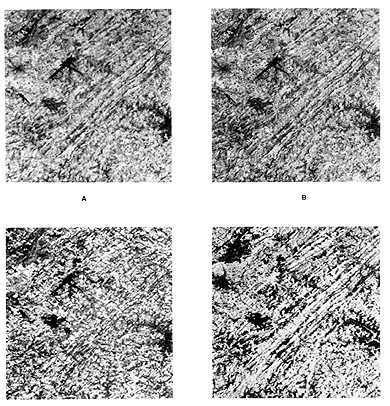
The upper left image is a MSS Band 7 rendition (stretched) of a June 1978 scene; the lower right is a linear stretch of a Band 7 of a February 1978 scene in which the ground was covered with snow. The upper right consists of a high bandpass filtering by Fast Fourier transform of the June subscene whereas the lower left is also a high bandpass filter version of Band 5, with Cubic Convolution resampling.
1-20: Which of the four subscenes seems best/worst
for picking out linear features? Compare the Fast Fourier and Cubic Convolution
processing for enhancing linear features and sharpening details. Make a guess
as to the identity (nature) of the irregular feature (in medium to dark gray)
that lies just south of the reservoir lake. ANSWER
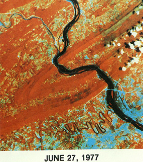
Now, back to Harrisburg and Gypsy Moth defoliation. Look at this June 27, 1977 subscene. The
defoliation appears as very dark gray patches on the ridges.
There are several ways to focus on this defoliation while ignoring other features/classes in the image. One is to calculate the Vegetation Index for the image. At least six different formulae have been proposed for this VI. We will use the simplest, namely, a ratio of MSS7/MSS5. When this is done there will be a range of DNs that could be shown as gray levels. But, another way is to produce a color mask image. All non-vegetated features are set to a single DN value (masking them out) and vegetated areas with signatures characteristic of trees and forest are assigned different colors. This is the result, with masked out areas shown in yellow-gray, healthy forest in green, defoliated forest in red, and stressed vegetation in purple.
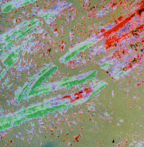
1-21: What is the advantage of this VI image? Where
may confusion occur? ANSWER
This same scene (and date) has been subjected to Principal Components Analysis. The first four component images are shown below (but, in an error in layout, the first component is B and the
second, A, with C and D the third and fourth components respectively.
1-22: Describe the main gray patterns in each component
image. ANSWER
A color composite can be made from any three of these images. Generally, the
fourth component image is bland and blurry and is not used. Here below is a
fcc image made using PC 2 = red; PC 1 = green; PC 3 = blue.
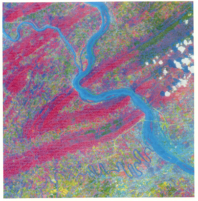
1-23: What does this PC image show that is less obvious
in the standard false color composite shown above? ANSWER
We are ready now to embark on supervised classifications of 4 areas within
the original full scenes that we have earlier examined. We'll start with this
8 class map of the Harrisburg subscene. This, and subsequent classifications
were all done on the IDIMS computer system at NASA Goddard.
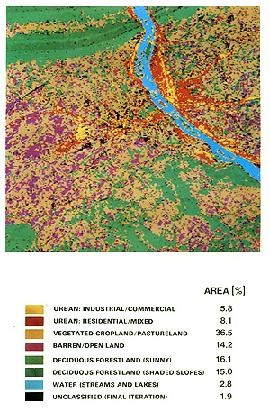
1-24: Evaluate this classification. ANSWER
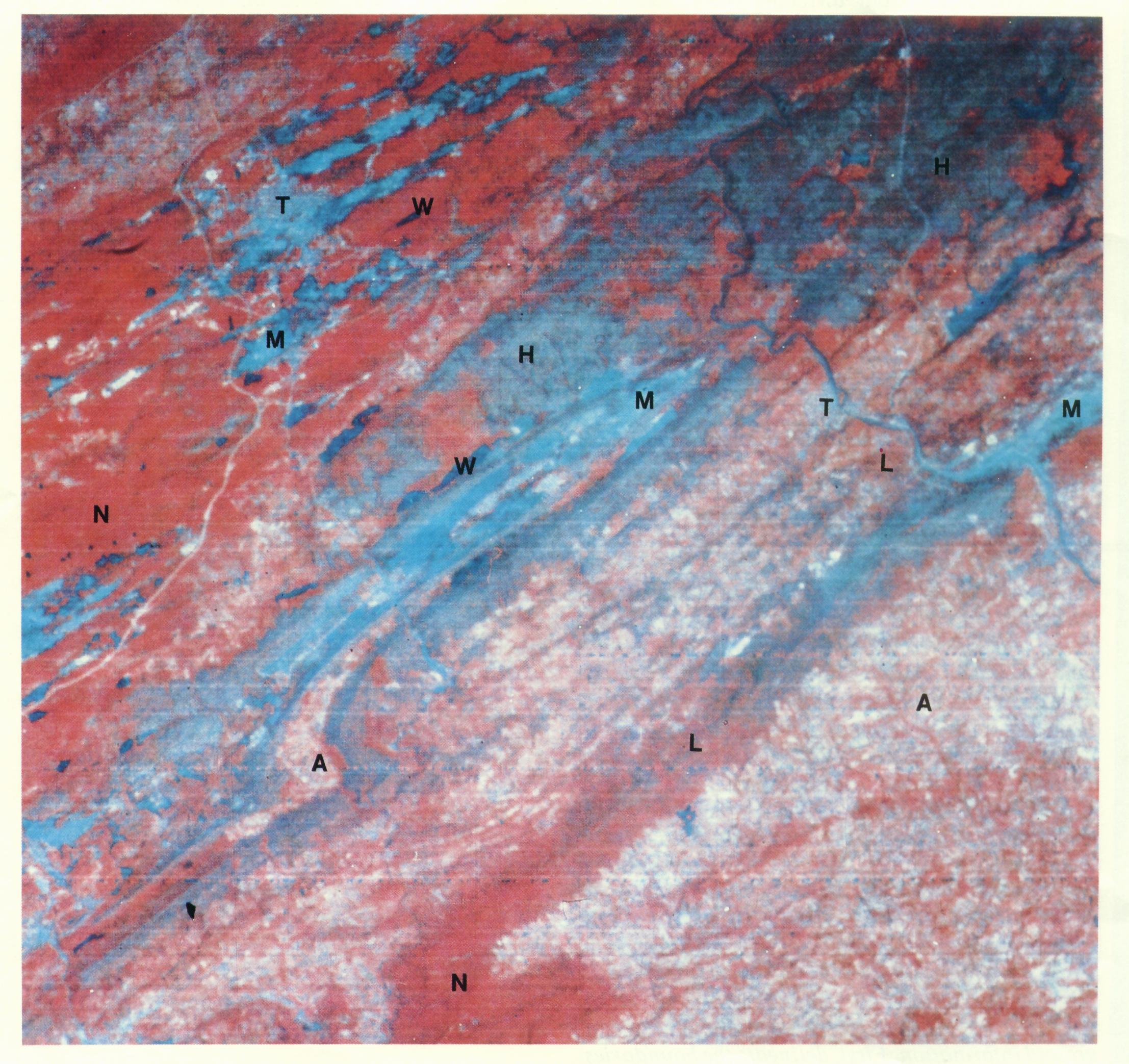
Onward to the anthracite coal belt. We present first a standard false color composite of the subscene that shows folded mountain ridges from Hazleton (T) southeast from Blue Mountain (lowest N) out into the
agricultural lands (A) of the Great Valley itself. Most of the brighter blue is mine waste. Defoliation was
moderate in this July 8, 1973 scene, being represented by the blue-gray tones.
A 1:78,000 scale black and white aerial photograph covers part of this Landsat
subscene.
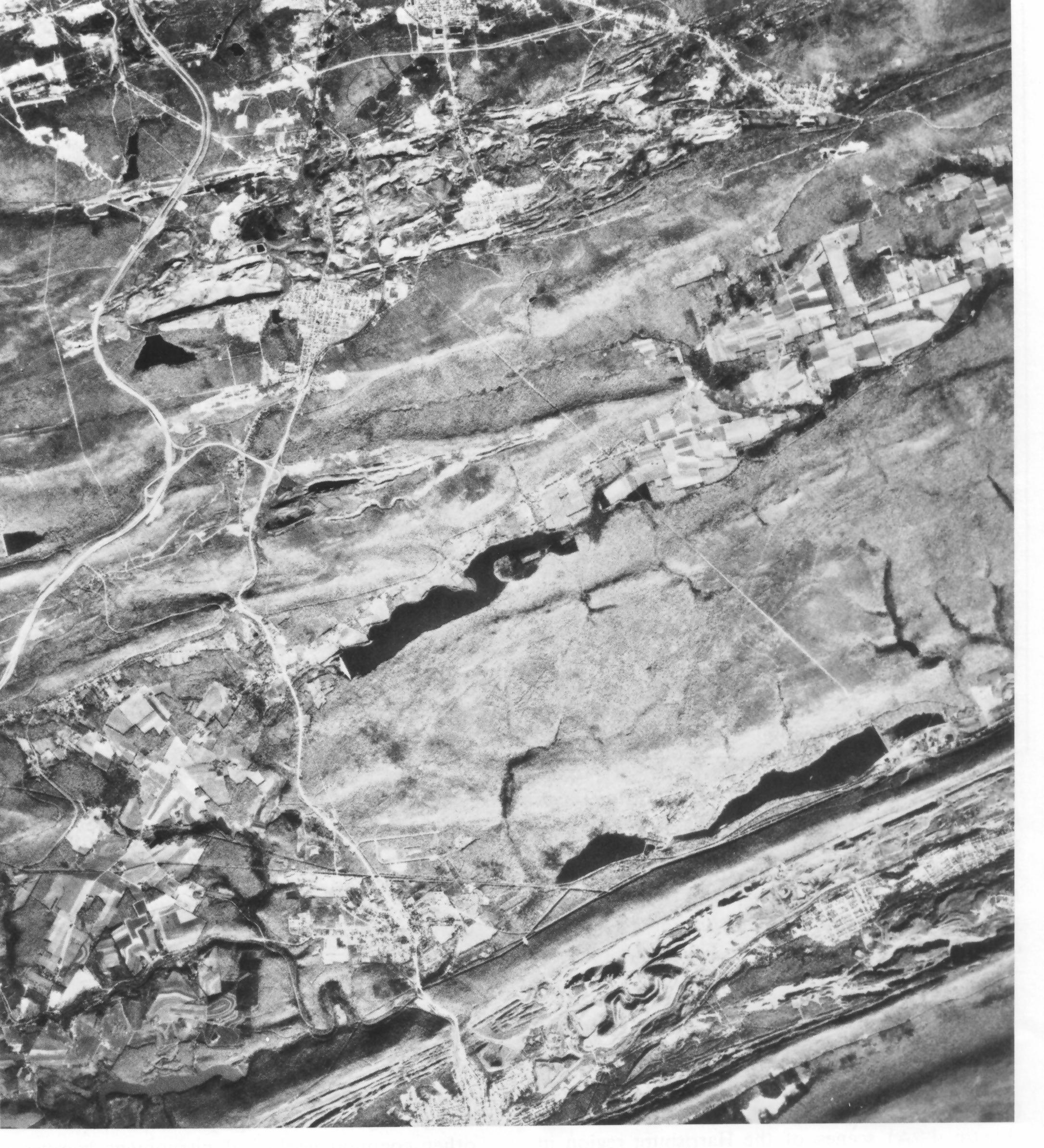
1-25: Try to fit this aerial photo into the Landsat
scene. Name the towns (use Atlas) you find. Is the mine refuse well displayed
in the photo. ANSWER
An unsupervised classification of the July 8th '73 scene was made on a General Electric Image-100 interactive processing system. Only four cluster classes were specified. After they were blocked out as patterns, they were then named, using the writer's general knowledge of the region. Here it is:
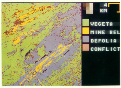
1-26: Evaluate this classification, compared with
your expectations from the fcc image for this date. Use the lakes (shown in
black) to relate the class map to the image. ANSWER
The next two classifications treat the area around the Chesapeake and Delaware Canal and Chesapeake Bay headwaters that occupy the lower right corner of the October, 1972 image.
The first of these is a supervised classification (right) of the subscene extracted
from the July 1977 full scene shown below on the left as a fcc image. The classes
were chosen by the writer following a field trip to the area and discussions
with the local Soil Conservation Service representative for New Castle County,
DE.
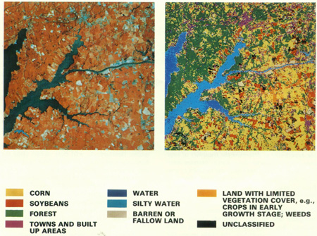
1-27: Which seems more abundant, corn or soybeans?
If you consult a map of the area, you might conclude that most of the larger
lavender patterns associate with towns and villages. But what about smaller
clusters of lavender; what might they be? Give a reason why so many of the fields
do not have straight boundaries, as is typical, nor are rectangular. ANSWER
The last classification shows categories of water purity in the Chesapeake
Bay headwaters in northern Maryland around Havre de Gras and Aberdeen. The date
of image acquisition was May 28, 1978. This is the result:
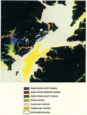
The mouth of the Susquehanna River is at center top. The Chesapeake Bay itself is the drowned segment of the lower Susquehanna which once emptied in Virginia near Norfolk but has been inundated by rising sealevel after the last glacial retreat. The land here is rendered black (except for white wetlands) by masking, which involves assigned all land pixels to a single value, given that color.
1-28: How do you think the turbidity in the Bush
River was determined (assessed)? ANSWER
We are nearing the end of this "exam". Now we turn our attention to two other types of remote sensors - those that produce active microwave - radar - images and those that measure thermal properties . These
sensor systems are treated in Sections 8 and 9 respectively. The following is just a preview.
For thermal imagery covering the Pennsylvania region and some neighboring states,
we will turn to the satellite known as HCMM (Heat Capacity Mapping Mission.
This operated during 1978 and produced scenes 700 km wide in three modes: Day
Visible; Day (thermal) IR; and Night IR.
Look first at a Day IR image (September 26, 1978) in which the bottom half includes much of the region
around Harrisburg that we have been studying. Dark tones correspond to "cool"; light to "warm".
1-29: First locate yourself within this image relative
to the landmarks you have come to know. Why are the ridges cool and the valleys
warm? There is a long, canoe-shaped white area in the right center; why does
it appear to be so hot? While it is not in the region you have been studying,
speculate on the very dark patterns in the upper center. ANSWER
Then, look at this Night IR image, obtained on June 11, 1978.
1-30: Why do the ridges and rivers and other water
bodies appear to be warmer (lighter toned) than the valleys? Can you find the
Harrisburg area? ANSWER
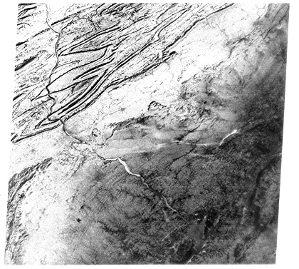
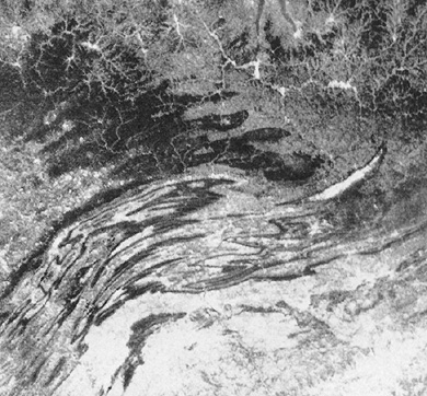
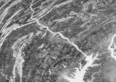
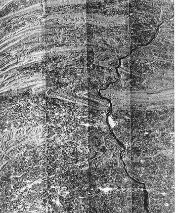
Finally, we take just a momentary peak at two radar images that include the Harrisburg area. Because interpretation of radar imagery requires considerable understanding of how the sensor operates and the
images are formed (which we will learn about in detail in Section 9), we will only show you the two examples and will not ask questions. But, we suggest you locate these images in the framework of the
Landsat scenes and pick out any special features and landmarks of which you are already familiar. The first image is made from an aircraft-mounted SLAR system (K-Band), as it flew over the terrain on July 22, 1966. The second was taken from space by the Seasat SAR on September 28, 1978. In that image,
the location of Harrisburg should be obvious (its buildings are strong reflectors).
Well, we've come to the end of this "exam". Rather challenging, but hopefully not tedious, eh! Grade yourself, but by merely working through it, you deserve an "A". In the rest of the Tutorial we will not again face such an extensive sequence of questions - just enough to help you become better acquainted with the important concepts and features associated with remote sensing interpretations.
Click here to get back to the last page of Section 1.